How-To Create a Normal Distribution Chart

My blog has moved to jimdehner.com 

Thank you for all the support over the past 2 years - I recently updated my blog to make it easier to read, improve the rendering of images and tie back to video presentations that are associated with the content - Check it out at  Jim's new blog  -   

How-To Create a Normal Distribution Chart

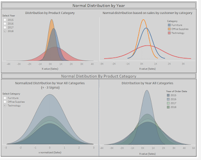
Occasionally there are Forum questions on creating normal distribution curves.  

The approach here relies heavily on the concept of data densification develop and refined by Bora Beran, Joe Mako, Jonathan Drummey, Ken Flerlage and others – Readers are encouraged to review their works on creating shapes and charts using the process.


This is a straightforward application of the normal distribution formula:
               

Y= (1/[σ*sqrt(2π])*e

Where  σ= Standard Deviation

                µ=Mean

You may find more elegant approaches – when you do please let me know so we all can benefit

The data used here is the “Superstore” data set that comes with Tableau desktop –  while the data set is detailed down to the transaction level the examples here go to the Year/Category level – the concept can be adapted to any level in the Superstore data set or your own

Overview –

Tableau does not draw curved lines – so we simulate the familiar smooth bell curve of the normal distribution with a series of straight lines  on an X-Y Cartesian coordinate grid.  The densification process is used to create intervals on the X-Axis (Sales in these examples).  As the number of intervals increases the plot becomes less angular. There is a parameter to adjust the number of intervals – somewhere between 50-100 intervals produces a reasonably smooth curve –play with it using your own data to see what works for you

– At this point if you have not familiar with Data Densification

STOP

and review one of the resources noted above. 

Step 1 Prepare the data for densification

Duplicate the data set by creating a union of the data with itself. Tableau will create a Dimension "Table Name" that can be used to distinguish the original data set from the duplicate - in the example the original data set is "Orders" and the duplicate in "Orders1"

Next create a calculation to define the ends point needed for the X-values

Path =   if [Table Name]="Orders1" then 1 else [max number of intervals] end

                Where [Max number of intervals] is the parameter to vary the x axis spacing

Use the Path formula to create bins –

Set the Bin Size to 1 - it will be the increment on the "X-axis" - (note I changed the bin name to Padded)

 


Step 2 – Create the X-values using the bins to pad the data – NOTE I used a +- 4 sigma range 

First, determine the µ and σ values – the average and the standard deviation values in this example on Sales – but we want to be able to vary the results by year and by category

For that use an LOD’s to create the needed combinations of year and category and the widow function forces the calculation to be executed in each bin across the viz

Mu=  window_min( avg({ FIXED year([Order Date]),[Category] :avg([Sales]) }) )

                Sigma= window_min(min({ FIXED year([Order Date]),[Category] :STDEV([Sales]) }) )

Where  (index()-1) is the bin number (interval) on the x axis

                X-value = (-4*[sigma])+([index-1 ]*(8*[sigma]))/window_max(max([Path])) 

Step 3 – Solve the Normal Distribution formula for Y 

Table calculations are used to determine then Y value at each bin (x-value)

For clarity there are 2 calculations 

The coefficient = (1/[σ*sqrt(2π])

                                 Coeff= 1/(sqrt(2*pi()*([sigma]^2)))

The Exponent =
                            Exponent = (-((([X value (Sales)])-[mu])^2)/((2*([sigma]^2)))  )

And then combined them in a single formula for Y (note Tableau does not have an "e" function but the EXP() will return the correct value)
                                                

Y= ([coeff]*EXP([exponent]) )

Step 4 – Create the viz –

Place the X and Y values on columns and rows then add the Mu and Sigma values to the Detail tile

Then add Padded (the bins) to the viz and set the calculation across the bins (all places)

You can also make normalized distribution charts using the formula below

                x-normalized = ([mu]-[X value (Sales)])/[sigma]

and replace the x-value in any of the charts

 
Finally, I added a parameter and a filter to allow the user to change the number of standard deviations visible in the charts
               
 N-Std Dev Filter =  [x normalized (Sales)] >= -[enter number of standard deviations] and              [x normalized (Sales)]<=[enter number of standard deviations]


Place it on the filter shelf – it too is a table calculation set to use Padded – then set to True 

The workbook containing these examples and more can be found on my Tableau Public site at https://public.tableau.com/profile/jim.dehner#!/vizhome/Howtocreateanormaldistributionchart_v2018_3/summary

Jim